Optimizing a simple analog filter for any PWM

Analog
2023-09-23 21:19:52

Recently there have been a series of design ideas published based on the topic of “processors” of PWM signals. The purpose of these processors is to minimize both the settling time in response to a PWM duty cycle change and the residual PWM ripple. In many cases the simpler processors—which consist only of a low pass filter built with resistors and capacitors—perform well (Figure 1).

Wow the engineering world with your unique design: Design Ideas Submission Guide

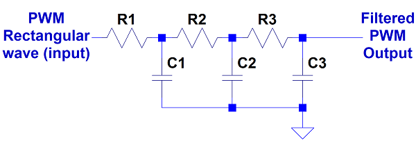
Figure 1 Simple PWM processor with a low pass filter built with resistors and capacitors, this filter structure can implement real poles only.

Advancements in LED Drivers for Next-Generation Automotive Exterior Lighting09.18.2023

Reducing the Production Cost of Integrated Circuits in the Integration Era09.14.2023

Democratizing Edge AI and ML with a No Code Approach09.12.2023

However, there has been little discussion on how to select optimal filter component values for PWMs of arbitrary characteristics, let alone for the specific PWM (8-bit, 1MHz clock) mentioned in one idea. In this article, I’ll describe a method for the optimization of these simpler filters for PWMs of arbitrary periods.

Let’s start with some nomenclature: we’ll characterize the unfiltered PWM as having B bits, a duty cycle d, a period T, and (unitless) output values of either 0 or 1. (Warning: If you just want the solution to the problem and don’t want to experience the thrill of derivation and the agony of the math, skip to the “Implementing the solution” section at the end of this post.)

For any third order filter with negative, unequal poles p1, p2, and p3, the time domain response to a unit step is:

The response is different if two or three poles are equal. For three, it’s:

One of our interests is in the time (ts) it takes to settle to a specified fraction F of 1 (the worst case of a full scale PWM transition from d = 0 to 1). It is preferable to deal with the amplitude settling error (ASE), h(t, p1, p2, p3) = 1 – hh(t, p1, p2, p3). The ASE is completely settled (goes to zero) at time t = infinity. We might ask the value of ts such that h(ts,p1,p2,p3) = F = 2-B-1, or ½ LSB of the PWM. Of course, other choices can be made if an application produces smaller maximum duty cycle steps.

We’re also interested in the amplitude of the filtered PWM ripple. The filter’s frequency response is:

where j = (√-1) and ω is the frequency in radians/second (rad/sec).

The unfiltered PWM output can be represented as the sum of an infinite number of sinusoids of frequencies which are integral multiples of 1/T = ωPWM/(2π) Hz. The highest amplitude sinusoid that can be produced has a peak magnitude of 2/π when d = 50% and a frequency of ωPWM rad/sec. The entire PWM signal passes through a low pass filter which attenuates the higher multiples more than the first. Under these conditions, the output of a reasonably good low pass filter consists almost entirely of the frequency of ωPWM. It’s apparent that excessive ripple and excessive settling times are equally capable of ruining your day. So we seek to know the ωPWM and ts for filters such that the ASE and the ripple amplitudes are both equal to F, that is, they meet “the criteria” that H(ωPWM, p1, p2, p3) = π∙HH(ωPWM, p1, p2, p3)/2 = F and F = h(ts, p1, p2, p3). Of course, we also want to find filters which give us the smallest ts and ωPWM for a given value of F.

Let’s start by looking at the specific case of a PWM with a value T = 28/1 MHz = .000256 for which ωPWM = 2π/T = 24543. An obvious starting point is a filter of equal-valued resistors and capacitors. For the Figure 1 circuit, the frequency response transfer function is:

Setting every R to 1 Ω and every C to 1 F, a polynomial roots finder routine can be used to determine the three poles and the value of ω that satisfy H() = F = 2-8-1: -3.247, -1.555, -.1981 and 9.0699. To get the same attenuation at a frequency ωPWM, the poles are multiplied and the resistors divided by FSF = ωPWM/ω. Of course, these resistors and the 1 F capacitors are inconvenient to work with, to say the least. So, we can choose an impedance scale factor ZSF such as 10-8 to multiply the capacitances and divide the resistances. The results are 37.0k (select the nearest standard value) and 10n. (Applying a ZSF has no effect on the filter’s response.) Knowing the poles for the 1 Ω / 1 F filter and requiring that h( ) = F, a root finder routine also gives us a value of ts = 32.5 s. Dividing ts by FSF maintains the same F and results in a value of ts equal to 12.01 ms.

Of course, there is no reason to expect that equal R’s and C’s will produce a filter that yields the lowest possible ts and ωPWM for a given value of F. How shall we search for a better filter? We use Monte Carlo. Starting with FSF-scaled values of the poles above, a new, better pole set is selected only if it reduces the value of either H( , , , ωPWM) or h(, , , ts) without increasing that of the other. A 10 million sample Monte Carlo with sets of randomly chosen poles was run. The result was poles at -2290.7, -2238.9 and -2218.6, a better ripple attenuation of .001938 < F, and a vastly improved ASE of 7.3834∙10-10. Clearly, the best choice is identical poles, sometimes referred to as synchronous ones. Unfortunately, it’s impossible to implement synchronous poles with the Figure 1 network. But we can get close if we set R3 = K∙R2 = K2∙R1 and C1 = K∙C2 = K2∙C3, with K being a value greater than unity. The larger K is, the better. Of course, there are obvious practical limits to the value of K, but let’s look at cases where K is 1, √10, 10, 100 and infinity. See Figure 2, which shows the time domain responses of filters which meet “the criteria”.

Figure 2 The ASE is shown for a full scale PWM transition verses time for various filter types. The horizontal line corresponds to an ASE of 2-9.

The dashed horizontal line is at a value of F = 2-9. Each of the other curves corresponds to the ASE of a filter whose H( , , , ωPWM) is also F. The curves intersect the horizontal line at the time when the filter’s ASE falls to F. The worst performer is the red curve with equal R’s and C’s for K = 1. The yellow and green, for K = √10 and 10 are better and seem practical, but the blue K = 100 filter requires impedance ratios of K2 = 10000. And the violet K = infinity curve is unrealizable… or is it?

The filters of the Figure 1 network will degrade in accuracy when driving resistive loads. The simplest solution is to buffer their outputs with an op-amp in the voltage follower configuration. Using this op-amp has another big advantage: the filter configuration in Figure 3 expands the number of realizable filter types to include not only the equal pole version, but an even better performer—a complex pole filter that has been determined by trial and error, starting with the poles of a Bessel filter. The “better” poles are: -.84668, -.786203+.725726∙√-1 and -.786203-.725726∙√-1. This filter’s R values can be scaled so that its attenuation H( , , , ) at ωPWM is F. The scaled filter’s performance is reflected by the black curve. Why the odd shape? The complex poles yield a time response which consists of damped oscillations. It passes through zero repeatedly as it settles. What is graphed is the absolute value of the response.

Figure 3 Image of filter structure that can implement real poles (some or all of which can be identical) and complex ones. For the component values shown, the parameter values in each given row of the complex poles section of Table 1 are satisfied (see text).

You might think that these graphs show the innate superiority of the complex pole filter. But they only represent the case where “the criteria” are met for F = 2-9. What about for other values of F? What about other PWMs with values of ωPWM? Here’s an answer. PWM’s have an integer number of bits, so it makes sense to consider values of F = 2-N only for N being a set of positive integers. For each 2-N and each filter under consideration, we can identify values of ω and ts which meet “the criteria”. Knowing ω, an FSF can be calculated for any desired PWM’s ωPWM, and that FSF can also be used to determine the values of the scaled ts and the filter R’s. In a filter with the FSF-scaled poles, ωscaled = FSF∙ω and ts-scaled = ts/FSF. And so regardless of the PWM frequency ωPWM, the product of ωPWM and the FSF-scaled ts will remain constant. The smaller the value of this product, the better. We can compare these products for the complex and synchronous filters to determine which is the better choice for each value of F. Refer to Table 1.

Table 1 Values of ω, ts and ω∙ts of the complex and synchronous filters for various values of F = 2-N.

The comparison reveals that for every F, the complex filter has the smaller value product and is the better choice. We can now generalize the filter design procedure.

Implementing the solution

A specific example will illustrate the solution to the general problem. Assume a PWM where B = 8 and T = 2B/1 MHz = .000256. We want a ripple level and ASE of F = 2-9. Figure 3 shows the filter component values for the complex filter in Table 1. For N = 9, the filter gives a frequency of ω = 9.1868 for that value of F. But we want that attenuation to be at a frequency of ωPWM = 2π/T. We need to divide the filter’s resistors and the Table’s ts = 6.3876 by an FSF = ωPCM/ω = 2671.7. This yields R1 = 66.527 kΩ, R2 = 45.445 kΩ and R3 = 178.95 kΩ (you can use the nearest standard values) and ts = 2.39 ms. You might also choose to scale these capacitors and resistors by a constant ZSF, multiplying the resistors and dividing the capacitors by that value. The ZSF manipulation has no effect on the filter responses.

It should be noted that for values of N = 6 or less, the synchronous filter has a smaller, better value of ω than the complex one, and that for larger values of N, the values of ω are almost identical. The complex filter is still the better choice though; FSF’s can be calculated with values of ω in the denominator that are between pairs in the table. Making ω larger will increase ripple attenuation and the settling time. A value of FSF can always be found that will lead to smaller scaled filter values of ω and ts than those offered by the other filters.

Designing a filter for a PWM of arbitrary frequency

A method using an op amp and three pairs of resistors and capacitors has been presented for designing a filter for a PWM of arbitrary frequency and number of bits. This filter limits both the ASE and peak ripple to F, a user-selected negative integer power of 2. Filters with poles having various interrelationships were investigated. The selected complex-pole filter has the smallest product of frequency and settling time among those considered. Using Table 1 and Figure 3, the filter components can be scaled to the desired value of F for a PWM of any frequency. The same scaling can be applied to the settling time listed in the table to calculate the scaled settling time.

If you prefer an op amp-free solution, you might want to consider a K = 10 version of the Figure 1 circuit. With R1 = 4.3k and C1 = 100n, for an F = 2-9, the ts is approximately 4.6 ms that you see for the green curve in Figure 2. That filter’s ω is 15787 rad/sec for the same F. I have not provided a Table for this filter, but you can test the results in a circuit simulator when applying different FSF’s to the filter resistors.

Acknowledgements

I’d like to thank David Lundquist for the review of and the valuable suggestions that he provided for this article. Any errors that might have escaped notice are of course exclusively my own.

Christopher Paulhas worked in various engineering positions in the communications industry for over 40 years.